Using the AutoComplete feature

AutoComplete is a feature that is used to display a list of texts that have been put in the cell that is active. List of text will be displayed when entering new data if no initial letters (not necessarily 1 letter) with the same text that was typed in the active cell.

1. Create a new workbook (press Ctrl + N) and create data in the range A1: A3 as the example image below.

 
2. If you type P in cell A4 the AutoComplete feature will automatically display the man because the initial letters beginning with the letter P same Pria who had entered in cell A1.

 
3. Press the Enter key when the data you enter is the man. If the data you entered is not a man, then continue typing the data as usual.

AutoComplete feature is very helpful when entering many of the same data in a single column. However, there are some users who just do not like this feature because it makes the display AutoComplete sometimes we do not focus on entering data.

• Click the Office Button and then press the button Excel Options. Excel Options dialog box appears.

 

• Select the Advanced option. Remove the tick mark (√) the option Enable AutoComplete for cell values ​​and then press OK.
• To try it, type P in cell A4. If the man does not appear in the text cell A4, then was off in the AutoComplete feature.

insert Symbol

Not only in Microsoft Word, When creating reports using Excel sometimes we also need to enter a particular symbol. For example, the sigma (Σ) used debagai symbol for the number of the data series.

1. Click the tab Insert> Symbol Symbol dialog box then appears.

 
2. Select a symbol to be inserted into the cell and then press the Insert key. Do the same for the other symbol.

3. If no symbol to be entered, press the Close button.

 

Thus a brief description of my input data, may be useful for you all.

Undo and Redo feature in Microsoft Excel

After I explained briefly about Copying data in Microsoft Excel in a previous post, this time explaining what it is I kana Undo and Redo in Microsoft Excel.

Undo is a feature that is used to cancel orders that have been done before, while redo is used to repeat the Undo action ever canceled. Undo and Redo feature is not only applicable to input and edit the data. But you can also use the Undo feature to cancel the orders he had ever run, for example, you can cancel an order setting column widths before.

Here I will give three examples of the usefulness of the Undo and Redo:

1. To cancel orders that have been done previously contained Undo button in the Quick Access Toolbar, or press the key combination Ctrl + Z.

2. To cancel an order was made some levels simultaneously click the drop down button and select the Undo command to be aborted.

3. To repeat actions that have canceled Undo, Redo button or press the key combination Ctrl + Y.

That's the short explanation from me about Undo and Redo feature in Microsoft Excel, may be useful for you all.

Copying data in Microsoft Excel

After the previous post I have explained How to Edit and Delete Data In Microsoft Excel, this time I will explain how Copying data in Microsoft Excel. Ok, you can copy the data into a cell or range, if the data is already present on the cell or range to another. By copying the data, you do not need to type the same data over and over again so as to save time and effort.

1. Select the cell or range you want to copy. Select the Home Tab > Copy or press Ctrl-C. Cell or range you want to copy is marked with dashed lines.

2. Place the pointer on the desired cell, then select the Home tab > Paste or press the key combination Ctrl = V.

Similarly, a brief explanation of my About Copying the data in Microsoft Excel, maybe even Just a bit of explanation, but I hope to have very much to you all.

How to Edit and Delete Data in Microsoft Excel

There are 4 ways to emlakukan Edit and Delete Data In Microsoft Excel, the data you have entered into a cell sometimes not as expected. This can happen for many reasons, for example due to misreading or typo. Following steps to fix (edit) data in a cell:

1. Press the F2 key or double-click the cell you want to edit the data. Excel will then display the selected cell in edit mode.

2. Type the desired data and then press Enter. At the time of editing, press the Delete key to delete a character to the right of the insert. To erase the data on the left line insert, press the Backspace key.

3. In addition to the above, you can also edit the data by overwriting data with new data Lam. Place the mouse pointer on the cell you want to change the data. Type the new data, and then press Enter.

4. To delete data place the cell pointer to delete the data, and then press the Delete key on the keyboard.

May be useful for you all .... !!!!

Input Data in Microsoft Excel

Doing Before processing the data, you must first enter data into a cell. Following steps to enter data into a cell:

1. Select the cells that will be used to store data using a mouse or keyboard.

2. The process input data must be adapted to the type of data to be entered. The following provisions of the input data based on the type of data:

- Text. To enter text data as the data type when you type in a word processing application (Microsoft Word 2007), for example, type Computer sales data.

- Figures. To enter numeric data type in the data to be entered without the thousands separator.

If the data entered in the form of a decimal number, use a period (.) Or commas (,) depending on regional settings you use, for example, 125 414, 123.

To enter a negative number, enclose the number in parentheses () or a prefix number with a minus sign (-), for example, 125 414, 123

To enter a fractional number starts with a zero (0) and a space, then type a fractional number to be input. For example, to enter a fractional number 3/5 type 0 3/5

-Date. To enter data on use slashes (/) or hyphen (-) to separate the day, month and year, for example, to enter a date 5 September 2009 type 09/05/2009.

- Time. To enter data use a colon (:) to separate hours, minutes and seconds, for example, to enter the time at 10 over 32 minutes typing 10:32.

- Cell reference. You can enter the data from the reference cell address. Excess data from the reference cell address is the data will always be updated if there are changes in the source cells. You can also enter the data of the reference cell located in another worksheet.

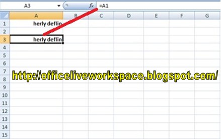
To enter data from a cell reference we type an equal sign (=) followed by the reference cell is used. For example, to enter data from cell A1, type = and then select cell A1 using the mouse or the keyboard naviasi. Cells used as a reference indicated by a dotted line. In addition, the formula bar will also display the address of the reference cell is used.

3. Enter data according to the type of data, and then press Enter. To cancel the data input, press the Esc key.

Protection Open and Modify Workbook in Excel

When saving a workbook, you can protect the workbook so that can not be opened or modified in any person. To open or modify the workbook, the user must enter the appropriate password.

Please see the following ropes:
 1. Click the Office Button menu and then Select Save to save the new workbook, or Save As to save the workbook with a different name. Will display the Save As dialog box.

2. Click the drop down button and select the menu Tools General Options.

 
3. Appears General Options dialog box. To protect the workbook can not be opened so that any person, enter the password in the Password to open text box:

4. To protect a workbook that can not be modified any person, enter the password in the password text box to modify: Press the OK button.

 
5. Confirm Password dialog box appears. Enter the password used to protect open workbook. Press the OK button.

6. Confirm Password dialog box appears. Enter the password used to protect modification workbook. Press the OK button.

7. Save As dialog box appearing. Type a file name in the File name text box: and then press the Save button. Each open workbook protected, Password dialog box appears as shown below.

 
8. At the prompt Password:, type the password you will enter when protecting the workbook. Press the OK button.

9. If you are using correct password, the password dialog box appears to open the workbook protection modifications.

10. At the prompt Password: type the password that you enter when protecting the workbook. Press the OK button. If you enter the correct password, workbook modifications can be made.

11. If you forget the password used to protect, press the Read Only to open the workbook. If there is a change in the contents of the workbook, save the workbook with a different name.

So first a brief description of my protection and Modified Open Workbook in Excel. May be useful for you. And that certainly saay will give the other tutorials on post-post next.