Well, according to the title of this post I will be explaining the message Input Method validation data in Microsoft Excel. Following on the previous post I have explained How to perform Data Validation Settings in Microsoft Excel.
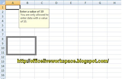
Input Message is the information that can be presented to users about what data should or should not be included in the validated cell. Information is displayed by default when the user selects a validated cell.
1. Blocks that have been validated range (A1: A5). Select the Data tab> Data Validation> Data Validation. Dialog box will appear and select Data Validation Input Message tab.
2. Tick mark (√) in the Show input message when cell is selected to display the Input Message validated when a cell is selected.
3. In the Title text box: type the title information data validation, for example, type Enter a value of 10.
4. Input message in the text box: type of data validation information. For example, type You are only allowed to enter the data with a value of 10.
5.If the settings are finished press the OK button. Select a cell in the range to be validated, for example cell A1. Input Message will appear as shown below.
By default the Input Message displayed at the bottom of the cell to be validated. To change this, click and hold the left mouse button on the Input Message. Drag the Input Message on the position you want. If it is appropriate, release the left mouse button.
A few of my brief explanation of the message Input Method validation data in Microsoft Excel, May be useful for you all. Do not forget to look forward to other Excel tutorials.
Tutorial Excel
Is a Complete Guide for those who still Layman with Excel 2007. Preparation of material practice than theory put forward in the hope of making you become really proficient at using Excel 2007.
How to perform Data Validation Settings in Microsoft Excel
In the Older Post I Already Gives Explanation On How To Edit Data Using the Replace Feature in Microsoft Excel, this time I will give further explanation of the Data Validation Settings in Microsoft Excel.
Data Validation settings is relatively easy because we only live determines what data should the user entered into a cell to be validated.
1. Press Ctrl + N to create a new workbook. Block cell or range to be validated, in this example the block range A1: A5.
2. Select the Data tab> Data Validation> Data Validation dialog box will bring up the data validation.
3. To perform the validation settings tab select settings. In the box Allow choice: you can choose the following options are available:
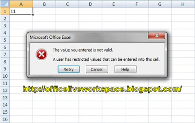
6. To test the data type in cell A1 with a value other than 10, eg 11. Warning message box will appear as shown below.
Values used in setting the Validation of data can also be derived from the reference cell. With these settings, the validation will always adjust the value contained in the reference cell is used.
1. For example, we will use cell B1 as a reference cell in the Data Validation. Type 10 in cell B1.
2. Block range A1: A5. Select the Data tab> Data Validation> Data Validation. Will Data Validation dialog box appears.
3. Select the Settings tab and then select Whole number on the box Allow option: In the Data option: select equal to. Type = B1 Minimum text box: as in the picture below.
Thus a brief explanation from me about How to Setup Data Validation in Microsoft Excel, may be useful for you all.
Data Validation settings is relatively easy because we only live determines what data should the user entered into a cell to be validated.
1. Press Ctrl + N to create a new workbook. Block cell or range to be validated, in this example the block range A1: A5.
2. Select the Data tab> Data Validation> Data Validation dialog box will bring up the data validation.
3. To perform the validation settings tab select settings. In the box Allow choice: you can choose the following options are available:
- Any Value. If you choose this option, then the user is allowed to enter any value without any restriction.
- Whole number. If you choose this option, then the user is only allowed to enter data such as numbers.
- Decimal. If you choose this option, then the user is only allowed to enter decimal data.
- List. If you choose this option, then the user is only allowed to enter the data on the list. The list can be derived from a cell reference or you enter directly into the Data Validation dialog box.
- Date. If you choose this option, then the user is only allowed to enter the data date.
- Time. If you choose this option, then the user is only allowed to enter time data.
- Text length. If you choose this option, then the user is only allowed to enter a long text data with certain characters.
- Custom. If you choose this option, then the user is only allowed to enter the data set using the formula.
- Between. If you choose this option, then the user is only allowed to enter data with a minimum value to the maximum value that you specify.
- Not Between. If you choose this option, then the user is not allowed to enter data with a minimum value to the maximum value that you specify.
- Equal to. If you choose opasi, the user is only allowed to enter data with the value you specify.
- Not equal to. If you choose this option, then the user is not allowed to enter data with the value you specify.
- Greater than. If you choose this option, then the user is only allowed to enter data with a value greater than the value you specify.
- Less than. If you choose this option, then the user is only allowed to enter data with a value less than the value you specify.
- Greater than or equal to. If you choose this option, then the user is only allowed to enter data with a value greater than or equal to the value you specify.
- Less than or equal to. If you choose this option, then the user is only allowed to enter data with values less than or equal to the value you specify.
6. To test the data type in cell A1 with a value other than 10, eg 11. Warning message box will appear as shown below.
Values used in setting the Validation of data can also be derived from the reference cell. With these settings, the validation will always adjust the value contained in the reference cell is used.
1. For example, we will use cell B1 as a reference cell in the Data Validation. Type 10 in cell B1.
2. Block range A1: A5. Select the Data tab> Data Validation> Data Validation. Will Data Validation dialog box appears.
3. Select the Settings tab and then select Whole number on the box Allow option: In the Data option: select equal to. Type = B1 Minimum text box: as in the picture below.
Thus a brief explanation from me about How to Setup Data Validation in Microsoft Excel, may be useful for you all.
How to Edit Data Using the Replace Feature in Microsoft Excel
In
the previous post I have explained How to Search Data in Microsoft Excel, so in this post I will discuss about How to Edit Data Using the Replace Feature in Microsoft Excel.To edit existing data in one or two cells alone would be easy for us to do. It only became difficult when we have to edit the data present in many cells. In this example, I will explain how we replace all data Male became Man.
1. Create a New Workbook (Press Ctrl + N) and then make the data as the example picture I've provided below.
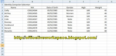
2. If you do not select a particular range, then edits the data will be applied to the whole cell. In this example the block range D3: D10 that means edit only applied in the range D3: D10.
3. Select Tab Home> Find & Select> Replace (Press Ctrl + H). Will Appear Find and Replace dialog box Replace tab.
4. Type the text that will be replaced in the Find what text box: In the Replace with text box: type in the new data that will be used. If so, press the Replace All to replace all the text in the range that we choose. Then the dialog box will appear as shown below.
5. A message box provides information that Excel has done a search and replacement in accordance with the provisions of 5 data that you set. Here I replace Male to Man, and then press the OK button.
In addition to changing the data in the entire worksheet or a selected range, you can also change the data contained in the entire workbook. For example, data man in the previous case, we will replace it not only contained in one worksheet.
1. Select the tab Home> Find & Select> Replace (or press Ctrl + H). Dialog box will appear Find and Replace - Replace tab.
2. Press the Options >> so the display Find and Replace dialog box will be as shown below.
3. Type the text that will be replaced in the Find what text box: Replace with text box: type in the new data that will be used. Select the workbook in korak Within option: Press the Replace All.
4. Confirmation box will appear again, then press the OK button. If Excel can not find the data that should be replaced, it will display a message box as shown below.
Thus a brief description of me on How to Edit Data Using the Replace Feature in Microsoft Excel, May be useful for you all.
1. Create a New Workbook (Press Ctrl + N) and then make the data as the example picture I've provided below.

2. If you do not select a particular range, then edits the data will be applied to the whole cell. In this example the block range D3: D10 that means edit only applied in the range D3: D10.
3. Select Tab Home> Find & Select> Replace (Press Ctrl + H). Will Appear Find and Replace dialog box Replace tab.
4. Type the text that will be replaced in the Find what text box: In the Replace with text box: type in the new data that will be used. If so, press the Replace All to replace all the text in the range that we choose. Then the dialog box will appear as shown below.
5. A message box provides information that Excel has done a search and replacement in accordance with the provisions of 5 data that you set. Here I replace Male to Man, and then press the OK button.
In addition to changing the data in the entire worksheet or a selected range, you can also change the data contained in the entire workbook. For example, data man in the previous case, we will replace it not only contained in one worksheet.
1. Select the tab Home> Find & Select> Replace (or press Ctrl + H). Dialog box will appear Find and Replace - Replace tab.
2. Press the Options >> so the display Find and Replace dialog box will be as shown below.
3. Type the text that will be replaced in the Find what text box: Replace with text box: type in the new data that will be used. Select the workbook in korak Within option: Press the Replace All.
4. Confirmation box will appear again, then press the OK button. If Excel can not find the data that should be replaced, it will display a message box as shown below.
Thus a brief description of me on How to Edit Data Using the Replace Feature in Microsoft Excel, May be useful for you all.
How to Search Data in Microsoft Excel
After the previous post I have explained How to create a list in Microsoft Excel Data Series. This time I will explain how to search data in Microsoft Excel. Excel 2007 has billions of cells in each worksheet. To find the data one by one in each cell it will take a lot of time and effort. To overcome these problems, you can use the Find feature to speed up the search process the data.
1. Select the tab Home> Find & Select> Find. (Or press Ctrl + H). Find dialog box appears you Find Replace tab.
2. Type of data to be searched in the Find What text box: If the data to be searched had been previously entered, click the Find What drop down list:
3. Press the Find Next button. If the data you are looking for is found, then the data will be selected. However, if the data you are looking for is not found, a message box will appear as shown below.
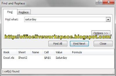
4. Press the back button Find Next to search for the same data later. So that we do not need to press the Find Next button repeatedly, press the Find All to conduct a search all data at once. The result will be as shown below.
5. Click one of the lines of the search results. Cells containing the data you are looking for then be selected. If the search data is completed press the Close button.
A few of my brief explanation on How to search the data in Microsoft Excel, may be useful for you all.
How to create a list in Microsoft Excel Data Series
In addition to the data series number or date, you can also create a list of the data series itself. For example, you create a data series name of your company's employees. This technique would be very helpful if the data series are frequently used.1. Press Ctrl + N to create a new workbook. Click the Office Button and then press the button Excel Options. Excel Options dialog box appears.
2. Select the option line and press the Edit Custom List. Custom dialog box will appear List. Enter a series of data in the text box list entries: like the example image below.
3. If so, press the Add button. If there is no data series you'll make again press OK.
4. Will reappear Excel Options dialog box and then press OK.
5. To try typing Roy result in cell A2. Drag the fill handle in cell A2 down until cell A8. The result will be like this.
Listing data series can also be derived from the range that contains specific data. For example, you create a list of data series subsidiary contained in range A1: A10.
1. Press Ctrl + N to create a new workbook. Type a company branch data in the range A1: A10 as in the image below.
2. Click the Office Button and then press the button Excel Options. Excel Options dialog box appears. Select the option line and press the Edit Custom Lists. Custom Lists dialog box appears.
3. Import list in the text box cells: Type $ A1: $ A $ 10, the range of sources used in the data series.
4. The move can also be done by pressing the button on the right of the Import list box From cells: Collapse Options dialog will appear as shown in the example image below.
5. Block range A1: A10 (the block is marked with dashed lines) and then press the button.
6. Reappeared Custom Lists dialog box and then press the Import button. Range of data series that have been entered will look something like this.Press OK
7. Will reappear Excel Options dialog box and then press OK.
8. To try the American Branch of the result type D1. Pull Handle on cell D1 fill down until the cell D10. The result looks like this.
Similarly, a brief description of me on How to create a list in Microsoft Excel Data Series. May be useful for you all.
Making Series Serial Data In Microsoft Excel
Serial Data Series is a series of data most commonly used Excel users. Therefore, Excel provides a special technique to allow users to create data series number, for example using the key combination Ctrl to speed up the manufacturing serial number of the data series.
1. Press Ctrl + N to create a new workbook. Type the initial value of the data series in cell A2, such as type 1. Place the pointer in cell A2.
2. Move the pointer on the black frame in the lower right corner of cell A2 (fill handle). Click and hold the deed and then pull down the handle to the cell A11.
3. Range A2: A11 initially be charged the same data, ie 1. To transform the data into a series of sequential data click the AutoFill Options drop down menu and select Fill Series. As shown below.
To Make the serial number of the data series quickly use the Autofill feature in combination with the Ctrl key on the keyboard as you pull the Fill Handle. Type 1 into cell B2 as the initial value of the data series. Press and hold down the Ctrl key. Drag Fill Handle to cell B2 down to B11 cells. The result looks like the picture below.
You also can create a data series with a serial number of a certain multiples. For example, you create a data series starting from 1 to 15 in increments of 2.
1. type 1 as the initial value in cell C2. Because the serial number is any multiple of 2, type 3 into cell C3.
2. Block Range C2: C3 then drag the fill handle in cell C3 down to the desired value.
A few brief explanation of my series on How to Make Serial Data In Microsoft Excel, May be useful for you all.
Entering Data Using Pick From Drop Down List
Besides using AutoComplete feature, we can also display a list of previously entered text in the cells that are actively using the Pick From Drop Dwon List. According to the authors, this method is relatively easy because all the data displayed (not just the text that have the same initial letter).
1. Create a new workbook (press Ctrl + N) and create data in the range A1: A3
2. Place the cell pointer padaq A4. Click the right mouse button then select Pick From Drop Down List.
3. In cell A4 and then display a list of text that has been entered previously.
4. Select the data to be entered using the mouse or keyboard and then press Enter.
Here's my explanation of how sedikt Entering Data Using Pick From Drop Down List may be useful for you all.
Subscribe to:
Comments (Atom)


